\(T_{2}^*\) Ramsey with QPT

This experiment determines the dephasing time \(T_2^*\) by performing a Ramsey sequence combined with quantum process tomography (QPT).

Description

The dephasing time of a qubit, \(T_2^*\), can be extracted from a standard Ramsey experiment, which measures the decay of the population following a Ramsey sequence. In other words, it determines the diagonal elements of the density matrix, \(\rho\). This approach, however, ignores the off-diagonal terms, which contain information on the qubit's phase and coherence. The \(T_{2}^*\) Ramsey experiment described here extends the standard Ramsey experiment by using quantum process tomography (QPT) to recover these off-diagonal elements.

Diagonal and off-diagonal elements

In a two-level quantum system, the diagonal elements of the density matrix are given by \(\langle 0 | \rho | 0 \rangle\) and \(\langle 1 | \rho | 1 \rangle\), while the off-diagonal elements are given by \(\langle 0 | \rho | 1 \rangle\) and \(\langle 1 | \rho | 0 \rangle\).

To obtain the off-diagonal elements, it's necessary to know the expectation values of the Pauli-X and -Y matrices: \(\langle \sigma_x \rangle\) and \(\langle \sigma_y \rangle\), respectively. These are determined by measuring the qubit populations in each of the basis states and then calculating \(\langle \sigma_i \rangle\) (\(i=x,y\)) through

\[ \langle \sigma_i \rangle = P_{|1\rangle,i}-P_{|0\rangle,i} . \]

Here, \(P_{|0\rangle,i}\) and \(P_{|1\rangle,i}\) are the probabilities of measuring the state \(|0\rangle\) and \(|1\rangle\) in the Pauli-\(i\) basis, respectively.

The coherence function, \(W(t)\), can then be reconstructed through

\[ W = \frac{1}{2} (\langle \sigma_x \rangle - i\langle \sigma_y \rangle) = \frac{\langle 0 | \rho(t) | 1 \rangle}{\langle 0 | \rho(0) | 1 \rangle} = \langle e^{-i\phi(t)}\rangle, \]

where \(\phi(t)\) represents the accumulated phase due to fluctuations in the qubit's environment. These fluctuations are modelled as a stochastic process, \(\xi(t)\), which describes random variations affecting the qubit's phase over time. Specifically, \(\phi(t)\) is the integral of \(\xi(t)\) over the time interval \([0, t)\). The coherence function therefore describes how the qubit loses coherence over time. Because QPT reconstructs this complex coherence rather than relying on oscillating Ramsey fringes, it typically yields a more accurate — and often slightly longer — estimate of \(T_2^*\) than standard Ramsey.

Quantum process tomography

QPT is a method for reconstructing an unknown quantum process from measurement data. For more details, see Cross resonance QPT.

Experiment steps

1. A pulse sequence is applied to measure \(\langle \sigma_x \rangle\):

   1. A \(\frac{\pi}{2}\)-pulse (\(R_x(\frac{\pi}{2})\)) is applied to rotate the qubit around the \(x\)-axis, preparing it in a superposition state.

   2. A time \(\tau\) (free evolution time) is waited.

   3. A Hadamard gate (\(H\)) is applied to transform the qubit into the Pauli-X basis. In QruiseOS, since the Hadamard gate is not one of our native gates, we generate it using a \(\frac{\pi}{2}\)-pulse (\(R_y(\frac{\pi}{2})\)) followed by a \(\pi\)-pulse (\(R_x(\pi)\)).

   4. The resonator transmission is measured.

2. A pulse sequence is applied to measure \(\langle \sigma_y \rangle\):

   1. A \(\frac{\pi}{2}\)-pulse (\(R_x(\frac{\pi}{2})\)) is applied to rotate the qubit around the \(x\)-axis, preparing it in a superposition state.

   2. A time \(\tau\) (free evolution time) is waited.

   3. An \(S^\dagger\) phase gate and a Hadamard gate are applied to transform the qubit into the Pauli-Y basis. In QruiseOS, since these are not native gates, we generate them using a \(\frac{\pi}{2}\)-pulse (\(R_y(\frac{\pi}{2})\)) followed by another \(\frac{\pi}{2}\)-pulse (\(R_x(\frac{\pi}{2})\)).

   4. The resonator transmission is measured.

3. Steps 1 and 2 are repeated for different values of \(\tau\).

Analysis steps

1. The sweep parameter "delay" (\(\tau\)) is converted to total free evolution time (\(t\)) by adding half the duration of the \(\pi\)-pulse (\(t = \tau + \frac{t_\pi}{2}\)).

2. The expectation values of the Pauli matrices are calculated as a function of time. The qubit state is predicted from the \(I\!-\!Q\) data by applying the discriminator trained in the Readout discriminator training experiment.

3. The coherence function, \(W\), is calculated as \(W = \frac{1}{2} (\langle \sigma_x \rangle - i\langle \sigma_y \rangle)\). The result is normalised such that \(W(0) = 1\).

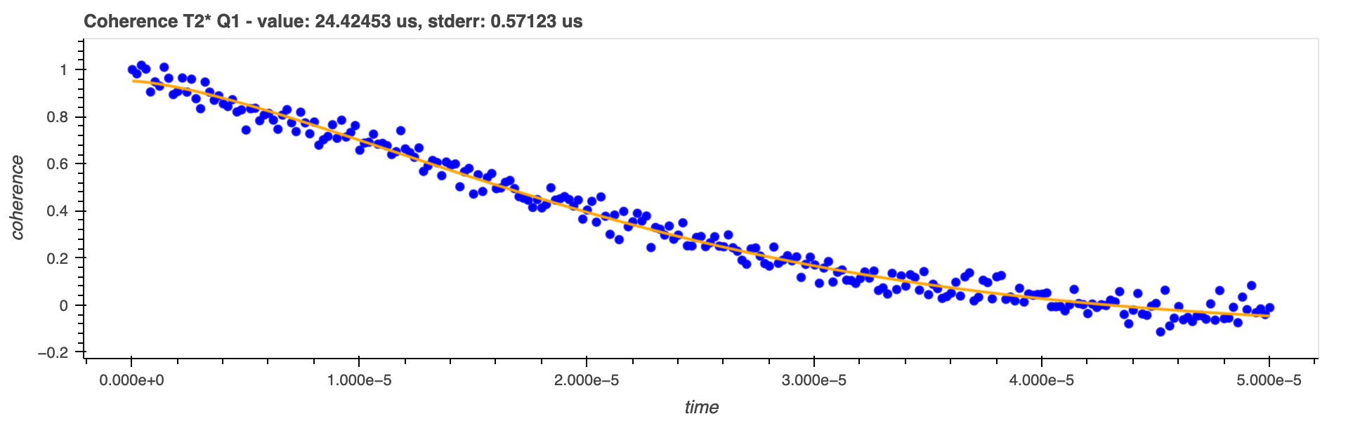
4. \(T^{*}_{2}\) is determined by fitting the stretched exponential function to the real part of the normalised coherence data: \(\(f(t) = A e^{-\left(\frac{t}{T^{*}_{2}}\right)^\alpha}\)\)

   The parameters in this function provide insight into the noise environment:

   • \(A\) (Amplitude): This represents the initial coherence value. It acts as a scaling factor and is not straightforward to relate directly to a specific physical parameter.

   • \(\alpha\) (Stretching exponent): This parameter characterizes the nature of the noise sources:

     • \(\alpha \approx 1\) (Markovian): Indicates fast, uncorrelated noise (white noise). This results in a simple exponential decay.
     • \(\alpha \approx 2\) (Gaussian/Non-Markovian): Indicates slow, low-frequency noise (typically \(1/f\) flux or charge noise).

   In superconducting qubits, we typically observe \(\alpha \approx 2\). This indicates that the dominant noise sources are slow (long correlation times). Because these noise sources are slow, their effects can be reversed (refocused) using a Hahn Echo sequence. This is why the dephasing time measured in a T2 Echo experiment is generally much longer than \(T_2^*\) in superconducting circuits.

If \(\langle \sigma_y \rangle \neq 0\)

If the noise is Gaussian, the imaginary part of the coherence, \(\langle \sigma_y \rangle\), should be equal to zero. The analysis currently fits only the real part of the coherence. If the imaginary part is significant, \(T^{*}_{2}\) may not be well-defined.