
Qubit–qubit coupling spectroscopy
This experiment measures the strength of qubit–qubit coupling as a function of qubit–qubit flux by fitting Rabi oscillations. The setup assumes a fixed frequency coupler and flux-tunable qubits.
Tunable coupler
For determining the strength of qubit–qubit coupling as a function of coupler flux, see Coupling spectroscopy.
Description
In a standard circuit QED (quantum electrodynamics) setup, qubit–qubit coupling can result from either longitudinal (along the qubit \(z\)-axis) or transverse (along the \(x\)- or \(y\)-axes) interactions. For transversely coupled qubits, the effective coupling Hamiltonian can be reduced to the excitation–exchange form under the following conditions1:
- The qubits are on resonance with each other.
- The rotating wave approximation is applied at the qubit frequency.
- If the interaction is mediated by a resonator rather than direct capacitive coupling, the resonator must be far detuned from the qubits (dispersive regime).
The qubit–qubit interaction Hamiltonian becomes
where \(g\) is the qubit–qubit coupling strength, and \(\sigma_i^{+}\) and \(\sigma_i^{-}\) are the raising and lowering operators, respectively, for the \(i^{\text{th}}\) qubit (\(i=A,B\)).
Physical realisation of transverse coupling
In practice, transverse qubit-qubit coupling can be engineered by either direct capacitive coupling, mutual coupling to a fixed-frequency coupler e.g. a resonator, or a tunable coupler. This last case is further explained in Coupling spectroscopy.
In this experiment, qubit A is prepared in its ground state and qubit B in its excited state. By sweeping the amplitude and duration of the flux pulse applied to qubit A, we briefly bring the qubits into resonance and induce Rabi oscillations between the \(|0_A1_B\rangle\) and \(|1_A0_B\rangle\) states, i.e. the populations of the two states oscillate in time at a frequency called the Rabi rate, \(\Omega\), given by
Here, \(\delta\) is the qubit–qubit frequency detuning and \(g\) is the coupling strength. At resonance, \(\delta=0\) and the Rabi rate reduces to \(\Omega=g\), allowing the coupling strength to be determined directly.
Experimental steps
-
Qubits A and B are initialised in their ground states, \(|0\rangle\).
-
A \(\pi\)-pulse (\(R_x(\pi)\)) is applied to qubit B to excite it to the \(|1\rangle\) state.
-
A flux pulse is applied to qubit A to bring its frequency close to that of qubit B. The amplitude and duration of the flux pulse are swept over a range around the expected qubit–qubit resonance.
-
For each combination of applied flux amplitude and duration, the two qubits are measured in their respective \(|0\rangle\) - \(|1\rangle\) bases via their readout resonators.
Analysis steps
-
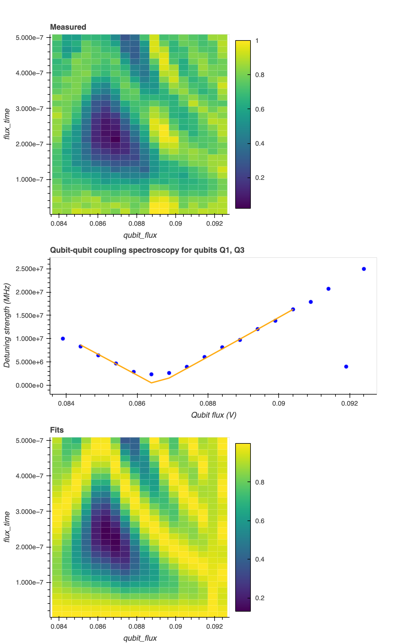
The qubit populations for the \(|0_A1_B\rangle\) and \(|1_A0_B\rangle\) states are computed as a function of the applied flux amplitude and duration (see top figure below). Here, the qubit states are identified from the \(I\)–\(Q\) data by applying the composite discriminator obtained in the Correlated readout error experiment.
-
For each value of flux amplitude, Rabi oscillations are fitted to the data of population against flux pulse duration, \(t\), using the function
\[ f(x) = 1 - a \left(\frac{g}{\Omega}\right)^{2} \sin^2(\Omega t). \]Here, \(a\) is a factor compensating for imperfect state preparation or measurement, and (as described above) \(g\) and \(\Omega\) are the qubit–qubit coupling strength and Rabi rate, respectively2.
-
The value for \(\Omega\) is extracted from each fit and plotted against flux amplitude. This is shown in the middle figure below.
-
At the minimum value of \(\Omega\), \(\delta=0\) and the coupling strength, \(g\), can be extracted by fitting a parabola to the data.
-
Alexandre Blais, Arne L. Grimsmo, S. M. Girvin, and Andreas Wallraff. Circuit quantum electrodynamics. Rev. Mod. Phys., 93:025005, May 2021. URL: https://link.aps.org/doi/10.1103/RevModPhys.93.025005, doi:10.1103/RevModPhys.93.025005. ↩
-
R. C. Bialczak, M. Ansmann, M. Hofheinz, E. Lucero, M. Neeley, A. D. O’Connell, D. Sank, H. Wang, J. Wenner, M. Steffen, A. N. Cleland, and J. M. Martinis. Quantum process tomography of a universal entangling gate implemented with josephson phase qubits. Nature Physics, 6(6):409–413, April 2010. doi:10.1038/nphys1639. ↩