Sessions: Simulation and optimisation

Once you've set up your system and your Problem is ready to go, you can run simulations and optimisations using a Session.

To create a Session:

from qruise.toolset.session import Session

sess = Session()

A Session provides the interface between your problem definition and the numerical solvers used to simulate or optimise the system.

Additional options

The examples below show only the most commonly used arguments. Methods such as evolve(), ensemble_evolve(), and optimise() support additional keyword arguments for controlling solver and optimisation behaviour. See the API reference for details.

Quantum simulations

To run a quantum simulation, you need to initialise your quantum simulation problem within the session:

sess.qsprob_init(prob)

where prob is an instance of Problem.

Once the problem has been initialised, you can use evolve to simulate the time evolution of the system:

data = sess.evolve("Tsit5", reltol=1e-3, abstol=1e-4, saveat=ts)

Here:

• "Tsit5" specifies the ordinary differential equation algorithm
• reltol and abstol are the relative and absolute numerical tolerances, respectively
• saveat specifies the time points at which the result is stored.

This returns an xarray.Dataset containing the simulation time points, quantum-state labels, and the simulated quantum states. Depending on how you defined the system, the quantum states are stored either as state vectors or density matrices.

Quantum optimal control

You may want to optimise your drive parameters to maximise the fidelity of a state preparation or gate operation. For this, you need to initialise the session with your quantum optimal control problem:

sess.qocprob_init(opt_prob)

where opt_prob is an instance of QOCProblem. You can then optimise the drive parameters using:

ps = sess.optimise("LBFGS")

where the optimisation algorithm is specified by the first argument. In this example, we're using "LBFGS", the limited-memory Broyden–Fletcher–Goldfarb–Shanno (L-BFGS) method.

Ensembles

Ensemble quantum simulations

QruiseML also supports ensemble simulations through EnsembleProblem. To initialise an ensemble simulation:

sess.ensemble_qsprob_init(ens_prob)

where ens_prob is an instance of EnsembleProblem. Then run the simulation using:

data = sess.ensemble_evolve("Tsit5")

The returned dataset contains the results for all ensemble members. This allows you to simulate an ensemble of initial states, Hamiltonians, parameter spaces, or time spans.

Ensemble quantum optimal control

For optimising an ensemble problem, use:

sess.ensemble_qocprob_init(ens_opt_prob)
ps = sess.optimise("LBFGS")

where ens_opt_prob is an instance of EnsembleQOCProblem.

Working with simulation and optimisation results

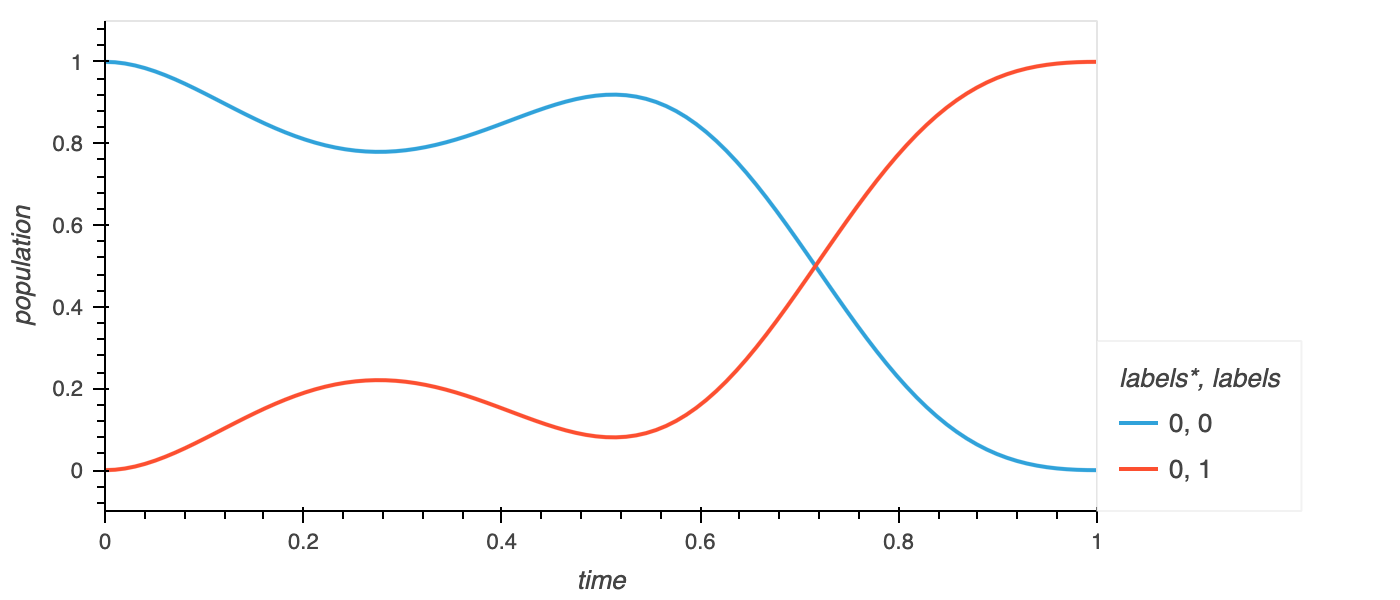
Additional quantities can be computed directly from the simulated quantum states and stored in the dataset. For example, the state populations can be added as a new variable:

data["population"] = np.abs(data["qstates"]) ** 2

The resulting population variable can then be used for further analysis or visualisation. For example, plotting the population against time:

import hvplot.xarray

data.hvplot.line(x="time", y="population").overlay().opts(legend_position="right")