Readout discriminator training (0-1 states)
This experiment trains a discriminator to determine which state a qubit is in.
Description
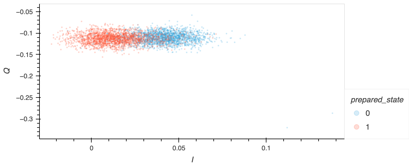
A Readout Discriminator can be trained to automatically determine a qubit's state from the \(I\) and \(Q\) values transmitted by its readout resonator. Each measurement on a qubit can be visualised using an \(I\)-\(Q\) plot (see below), where the blue and red circles correspond to the qubit being prepared in the ground or excited state, respectively.
You can see that (in this particular system) the first excited state (\(|1\rangle\)) tends to have a slightly larger \(I\) value than the ground state (\(|0\rangle\)). It's therefore possible to use the \(I\) value to determine which state the qubit is in. In other cases, it might be necessary to use both the \(I\) and \(Q\) values.
To train the readout discriminator, many time-integrated measurements of the \(I\)-\(Q\) values are compiled to statistically classify the qubit state. Often, the discriminator is used to classify only the 0-1 states, but it can also be trained for the 0-1-2 states (i.e., including the second excited state \(|2\rangle\)).
Initial Training vs Accurate Training
This experiment should be performed twice:
-
Initial Training: A first basic training of the discriminator uses uncompensated drive pulses with \(\pi\)-amplitude calibrated using Amplitude Rabi. This can be used for some initial experiments to obtain rough system parameters.
-
Accurate Training: A second, more accurate training of the discriminator uses DRAG-compensated pulses and \(\pi\)-pulses calibrated using ping-pong. By using these finely tuned drive pulses, the fidelity of preparing the \(|1\rangle\) state is enhanced, leading to a lower likelihood of misidentifying the state.
Enhancing Readout Contrast
In the example figure above, you can see that there's an overlap between the \(|0\rangle\) and \(|1\rangle\) states, meaning that sometimes the readout discriminator will determine the state incorrectly. To reduce the likelihood of this happening, a Readout Contrast experiment can be performed prior to Readout Discriminator Training.
Experiment steps
-
The resonator transmission is measured when the qubit is in the ground state \(|0\rangle\).
-
A \(\pi\)-pulse (\(R_x(\pi)\)) is applied, which prepares the qubit in the excited state \(|1\rangle\), and the resonator transmission is measured once more.
-
Steps 1 and 2 are repeated a large number (~1,000) of times in order to generate a sufficient number of points for each cloud.
0-1-2 Discriminator
The above instructions are for a 0-1 discriminator. If you want to also classify the second excited state \(|2\rangle\), replace step 3 with the following 2 steps:
3. A \(\pi_{12}\)-pulse (\(R_x(\pi_{12})\)) is applied, where the subscript denotes that the pulse is specifically designed for the \(|1\rangle \rightarrow |2\rangle\) transition, the amplitude of which can be determined using the Amplitude Rabi (1-2 states) experiment.
4. Steps 1-3 are repeated a large number (~1,000) of times in order to generate a sufficient number of points for each cloud.
Analysis steps
-
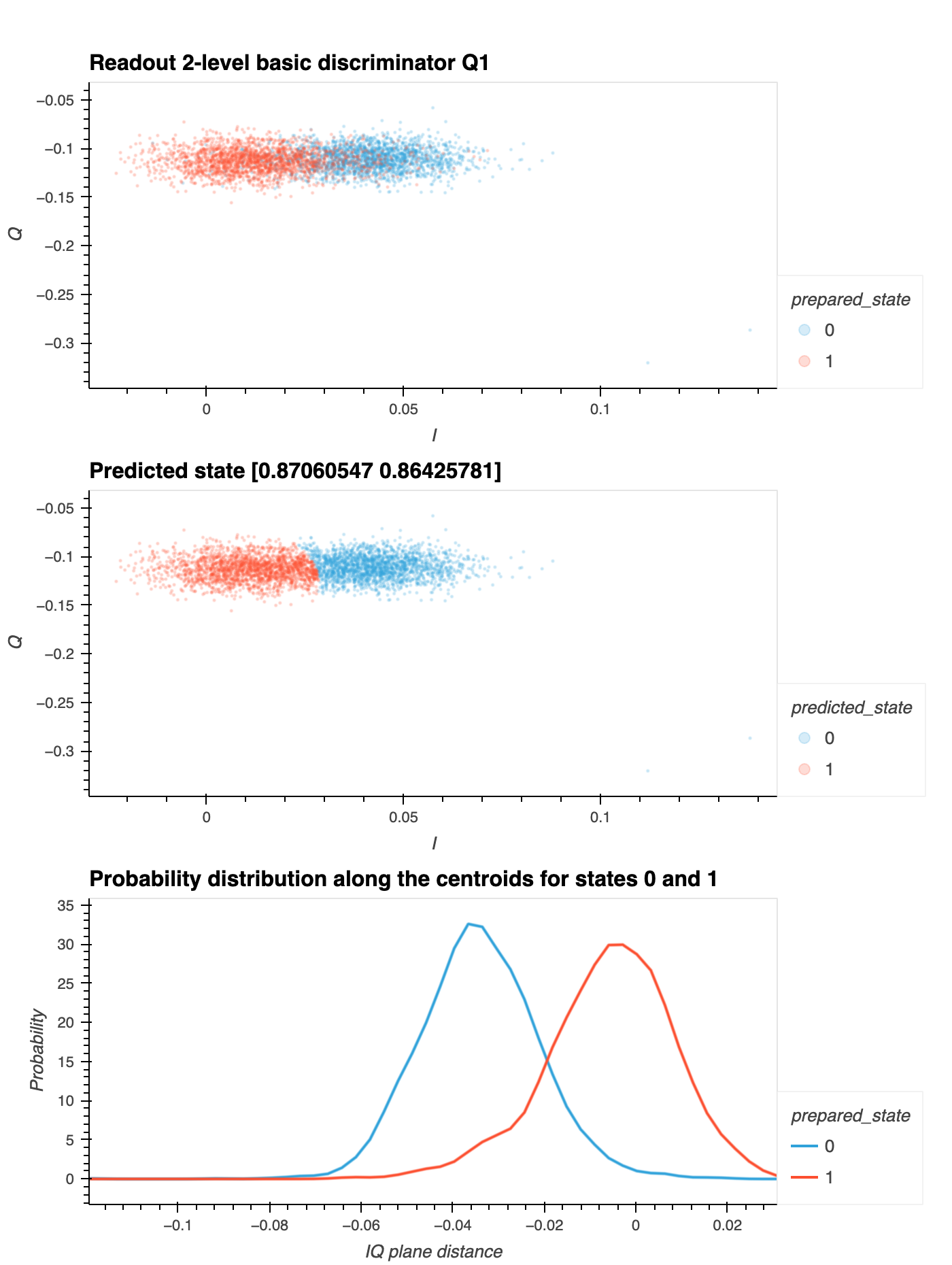
An \(I\)-\(Q\) plot is prepared (top figure below).
-
The discriminator is trained using Linear Discriminant Analysis (LDA) or Quadratic Discriminant Analysis (QDA), two well-known methods in supervised learning1. Thus, the conditional probability \(\text{P}(\text{state}_\text{measured}|\\ \text{state}_\text{prepared})\) is obtained for each state.
-
Option 1: This step is performed directly using the \(I\)-\(Q\) plot data. You can see in the middle figure below how the discriminator has assigned states based on the \(I\)-\(Q\) values.
-
Option 2: In reality, training the discriminator from the \(I\)-\(Q\) plot is often too complicated. As an alternative, the Probability Distribution Function (PDF) can be computed for each measured state along the axis that connects the centres of the \(IQ\)-cluster data and the discriminator can be trained using plot of PDF against \(IQ\) plane distance (see bottom figure below).
-
-
Benyamin Ghojogh and Mark Crowley. Linear and quadratic discriminant analysis: tutorial. 2019. arXiv:1906.02590. ↩

