Readout contrast (0-1 States)
This experiment tunes the amplitude (power) and frequency of readout pulses to increase the readout contrast for the \(|0\rangle\) and \(|1\rangle\) states of a qubit.
Description
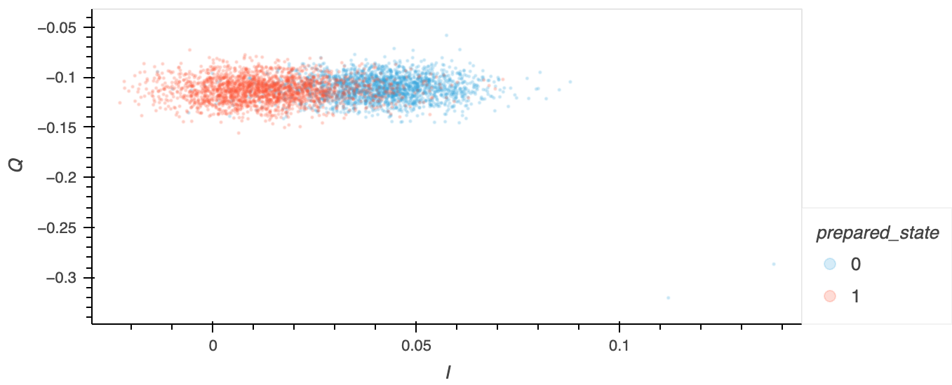
A Readout Discriminator can be trained to automatically determine a qubit's state from the \(I\) and \(Q\) values transmitted by its readout resonator. However, as described in the Readout Discriminator Training experiment, if there's an overlap between the \(I\)-\(Q\) clusters for the \(|0\rangle\) and \(|1\rangle\) states (see figure below), misidentification of the states can occur. By tuning the amplitude and frequency of the readout pulses, it's possible to reduce this overlap and enhance the readout contrast for more reliable state determination.
To identify the readout parameters that give the highest readout contrast, this experiment measures the \(I\) and \(Q\) signals transmitted by the resonator for different values of the readout pulse amplitude and frequency when the qubit is in the \(|0\rangle\) and \(|1\rangle\) states. The readout contrast can be quantified using the signal-to-noise ratio (SNR):
where \(\langle D \rangle\) represents the average distance between \(I\)-\(Q\) points corresponding to the \(|0\rangle\) state and those corresponding to the \(|1\rangle\) state, and Var(\(D\)) is the variance of these distances. In other words, the SNR – and therefore the readout contrast – is maximised if the \(|0\rangle\) and \(|1\rangle\) state \(I\)-\(Q\) clusters are small and far apart, i.e. they have no or minimal overlap.
Normality and Shapiro-Wilk Test
In the simplest approximation, one can just pick the amplitude and frequency combination that maximises the readout contrast. This works for the readout frequency, but the readout amplitude selected using this method is usually pretty high, which can lead to unintended qubit excitations (\(|0\rangle\rightarrow|1\rangle\) or \(|1\rangle\rightarrow|2\rangle\)). This is reflected in the \(I-Q\) plots losing their normality, which is a key requirement for the dispersive readout process.
In order to counter this loss of normality, the Shapiro-Wilk test1 is performed. The test statistic, \(W\), is a measure of how well the data fits a normal (Gaussian) distribution. The closer \(W\) is to 1, the more normal the data. The optimal readout amplitude is selected as the amplitude that maximises the readout contrast without going below a threshold \(W\) value, \(W_{th}\), which can be customised by the user.
Note
This experiment should be performed twice:
-
Initial tuning: A first basic tuning of the readout pulse parameters uses uncompensated drive pulses with \(\pi\)-amplitude calibrated using Amplitude Rabi. This can be used for some initial experiments to obtain rough system parameters.
-
Accurate Tuning: A second, more accurate tuning of the readout pulse parameters uses DRAG-compensated pulses and \(\pi\)-pulses calibrated using ping-pong to provide better contrast. By using these finely tuned drive pulses, the fidelity of preparing the \(|1\rangle\) state is enhanced, leading to a more effective determination of high-contrast readout parameters.
Experiment steps
-
The readout pulse amplitude and frequency are set to a given value and the resonator transmission is measured when the qubit is in the ground state \(|0\rangle\).
-
A \(\pi\)-pulse (\(R_x(\pi)\)) is applied, which prepares the qubit in the excited state \(|1\rangle\), and the resonator transmission is measured once more.
-
Steps 1 and 2 are repeated a large number (~1,000) of times in order to generate a sufficient number of points for each cloud.
-
Steps 1 to 3 are repeated for different values of the readout amplitude and frequency.
Analysis steps
-
The SNR and the Shapiro-Wilk statistic, \(W\), are calculated for each combination of readout amplitude and frequency from the \(I-Q\) data.
-
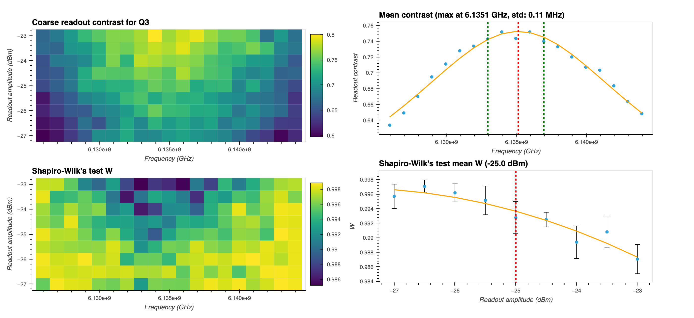
The SNR and \(W\) are each plotted as a colourmap on a 2D plot of readout amplitude against frequency (left panels in figure below).
-
The optimal readout frequency is obtained by fitting a Lorentzian to the contrast data after averaging over the readout amplitude. You can see for the data shown below, the optimal readout frequency \(\omega_r=\) 6.135 GHz (top right panel).
-
The mean of \(W\) (or median or minimum) is calculated for each amplitude value for a range around the optimal readout frequency. The optimal readout amplitude is chosen as the maximum whose mean \(W\) statistic doesn't fall below the threshold \(W_{th}\). You can see in the bottom right panel below that for a threshold \(W_{th}=\) 0.993, the optimal readout amplitude is -25 dBm.
-
Wikipedia. Shapiro–Wilk test. 2024. [Online; accessed 31-July-2024]. URL: https://en.wikipedia.org/wiki/Shapiro%E2%80%93Wilk_test. ↩

