Qubit-qubit coupling
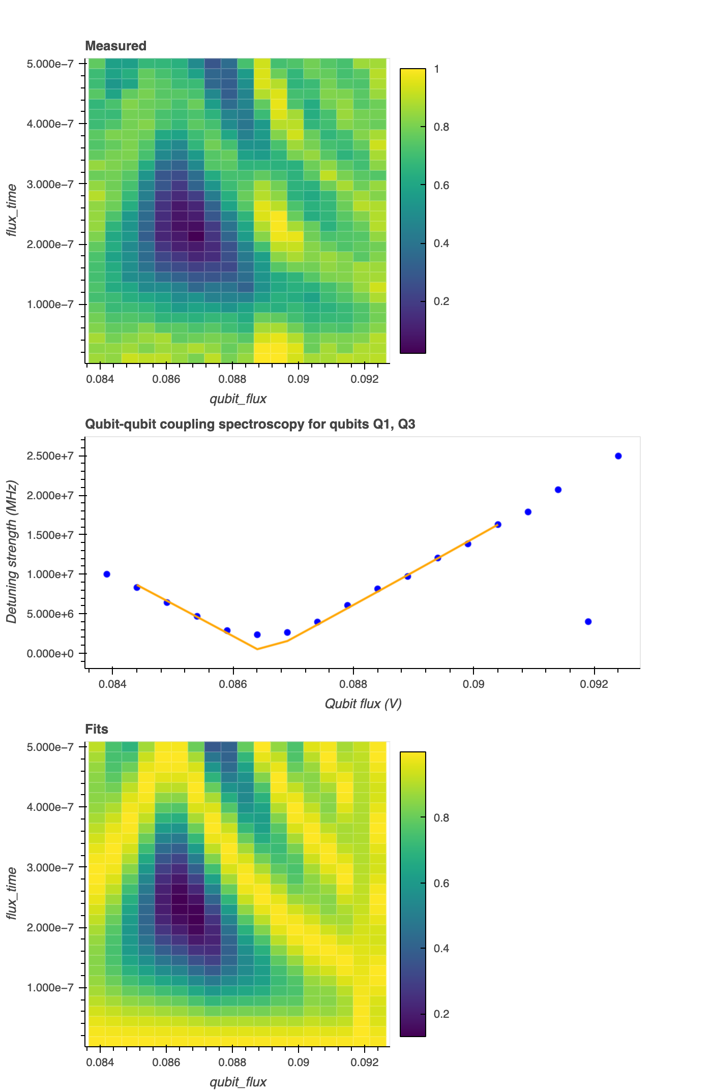
This notebook measures the strength of qubit-qubit coupling as a function of qubit-qubit flux by fitting Rabi oscillations.
Description
In a standard cQED setup, qubit-qubit coupling can result from either a longitudinal or transversal interactions. For transversally coupled qubits*, under certain conditions1, the coupling Hamiltonian can be described only by the excitation exchange interaction terms, i.e., \(H_{qq} = g (\sigma^{+}_{1}\sigma^{-}_{2} + \sigma^{-}_{1}\sigma^{+}_{2})\), where \(g\) is the qubit-qubit coupling strength. This experiment measures the transition frequency (and therefore the coupling) between the 01 and 11 qubit states. In this scheme, we consider two qubits A and B, with qubit A prepared in the ground state and qubit B in the excited state. By sweeping the amplitude and duration of the applied flux to qubit A, it is possible to bring both qubits into resonance and induce Rabi Oscillations between the qubit-qubit states, such as \(|g e\rangle\) and \(|e e\rangle\) (i.e., 01-11 states).
Experimental steps
-
Preparing the first qubit (qubit A) in the ground state \(|g\rangle\).
-
Applying a \(\pi\)-pulse (
RXGate(x)) to prepare the second qubit (qubit B) in the first excited state \(|e\rangle\). Note thatx = x180_amplitude. -
Sweeping the amplitude (
flux) and time duration (flux_time\(\equiv\)ts) of flux qubit A over a range of values defined around the expected values specified in the qubit parameters. For example, thefluxis swept in a range defined around the resonance flux (resonance_flux) between both qubits. The resonance flux is computed by minimizing the differenceresonance_flux = min( |qubit_freq_fn(f) - other_qubit_freq_fn(0)| )over a specified range using brute-force optimization. Here,qubit_freq_fnrepresents the frequency of qubit B as a function of the flux (f), whileother_qubit_freq_fnrepresents the frequency of qubit A. -
Measuring the resonator transmission and collecting the \(I\) and \(Q\) signals for each qubit
[0,1]and for each value offluxandflux_time.
Analysis steps
-
Computing the qubit populations 01-10 (
population) as a function offluxandflux_time. Here, we predict the qubit state from the \(IQ\) data by applying thecomposite_discriminatorobtained in the Correlated Readout Error experiment. -
Fitting Rabi Oscillations to the experimental trace (
populationversusflux_timefor eachflux). The function is \(f(x) = 1 - (g/\Omega)^{2} \sin^2(\Omega x)\). Here, \(\Omega = \sqrt{g^2 + \delta^2}\) corresponds to the Rabi frequency, i.e., the frequency at which the probability amplitudes of two energy levels fluctuate in an oscillating electromagnetic field. \(\delta\) is the detuning frequency (delta), and \(g\) is the qubit-qubit coupling strength (g). -
Determining the
resonance_fluxby fitting and minimizing a quadratic line shape to the spectroscopy trace (deltaversusflux). The fitting function \(f(x)\) follows a quadratic dependence as a function of the flux, i.e., \(f(x) = ax^2 + bx + c\), with \(x\) being the flux.
* In this architecture, the qubits can share either a capacitor or a tunable coupler. We shall explain this in the next notebook.
-
P. Krantz, M. Kjaergaard, F. Yan, T. P. Orlando, S. Gustavsson, and W. D. Oliver. A quantum engineer's guide to superconducting qubits. Applied Physics Reviews, 6(2):021318, 06 2019. doi:10.1063/1.5089550. ↩
