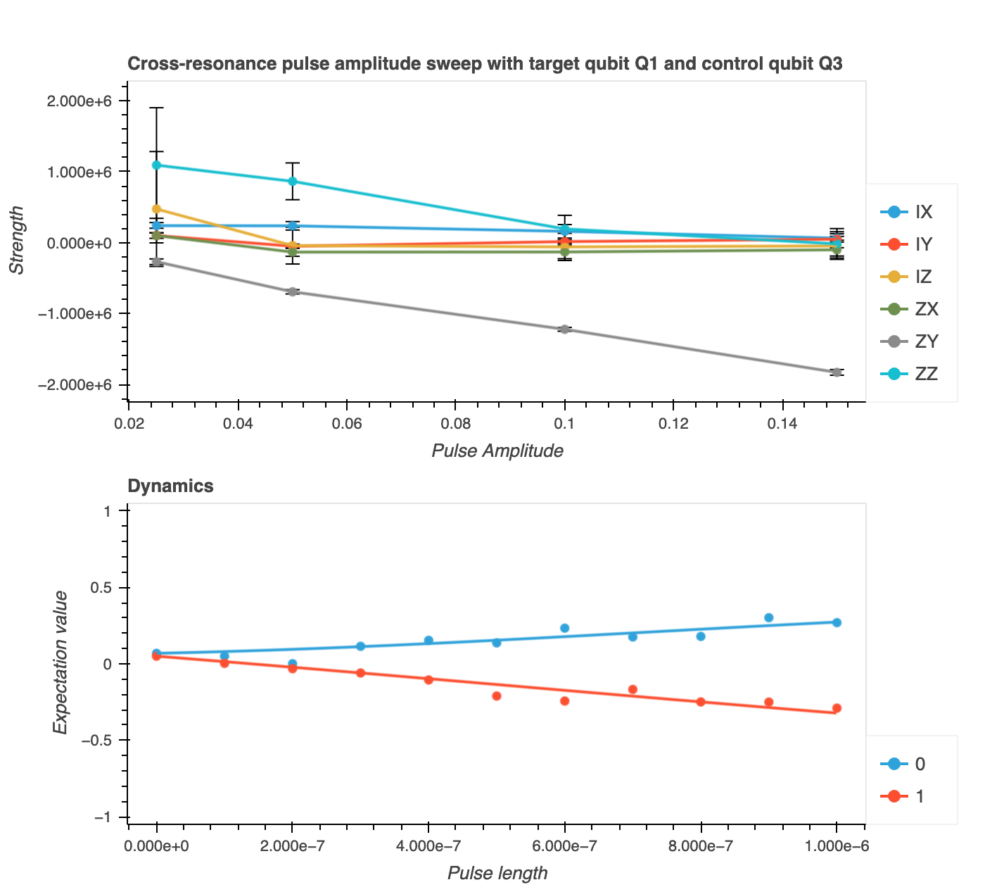
Cross resonance amplitude sweep
The notebook implements cross resonance by sweeping the control pulse amplitude and pulse duration
Description
In cQED, with a multi-qubit architecture, two-qubit entangling operations can be realized using microwave-activated cross-resonance interaction1. This interaction is enabled by the application of a cross-resonant drive tone, corresponding to a qubit drive resonant with a neighboring qubit's transition.
In the laboratory frame2, the Hamiltonian for the two-qubit system can be expressed as
Here, the first two terms describe the qubit Hamiltonians, while the last term represents the qubit-qubit coupling Hamiltonian. We can introduce a drive on the first qubit (referred to as the control qubit \(Q_{C}\)) at the transition frequency \(\Omega_{12}\) of the second qubit (referred to as the target qubit \(Q_{T}\)). In this scenario, considering the frame where both qubits rotate with the drive and under the condition \(g,\Omega_{12} \ll \Delta \omega_{12}\) (where \(\Delta \omega_{12} = \omega_{1} - \omega_{2}\)), the Hamiltonian \(H\) takes the following form:
where \(\{ \hat{ZX} = \sigma^{z}_{1} \otimes \sigma^{x}_{2}\),...} , and \(\epsilon\) is the cross-Kerr interaction term.
-
The off-resonant control qubit drive terms are defined as \(\Omega_{XI} = \Omega_{12} \cos(\theta_{12})\) and \(\Omega_{YI} = \Omega_{12} \sin(\theta_{12})\). They can be neglected when the drive amplitude \(\Omega_{12} \ll \Delta \omega_{12}\).
-
The cross-resonance interaction terms for the two-qubit system, \(\Omega_{ZX} = \mu \Omega_{12} \cos(\theta_{12})\) and \(\Omega_{ZY} = \mu \Omega_{12} \\ \sin(\theta_{12})\), are similarly dependent on the cross-resonance drive amplitude and phase but also the cross-resonance drive factor \(\mu\).
-
The rotations on the target qubit, \(\Omega_{IX} = \Omega_{12} \nu \cos(\theta_{12}) + \Omega_{12} m_{12} \cos(\theta_{12} + \phi)\) and \(\Omega_{IY} = \Omega_{12} \nu \sin(\theta_{12}) + \Omega_{12} m_{12} \sin(\theta_{12} + \phi)\), are given by the sum of the contribution from the quantum crosstalk characterized by the factor \(\nu\) and the classical crosstalk characterized by the factor \(m_{12}\) and relative phase \(\theta_{12}\).
-
See Ref 2 for further descriptions and definitions of the parameters mentioned here.
Using the results presented in Ref 2, we get the following effective Hamiltonian:
where \(\Omega^{T}_{CR}\) is a selected target rate at which to drive the cross-resonance interaction \(\hat{ZX}\).
From the previous descriptions, it is straightforward to see that the local drive on the control qubit (\(Q_{C}\)), resonant with the first transition frequency of the target qubit (\(Q_{T}\)), introduces an interaction between them. This interaction rate is proportional to the amplitude of the cross-resonant drive, \(\Omega_{12}\).
Experimental steps
-
Defining the circuits needed to perform cross-resonance tomography, the method
_build_single_qubit_ins-\tructionsinside the classCrossResonanceTomographyreceives qubit characterization and constructs a dictionary containing three key-value pairs:-
ctrl_rx180p: It creates a gate instruction namedrx180pfor the control qubit. The frequency is set to the value obtained from the characterization. -
target_rx90p: It creates a gate instruction namedrx90pfor the target qubit. The frequency is set to the value obtained from the characterization, and thexy_angleis set to0. -
target_ry90m: It creates a gate instruction namedry90mfor the target qubit. The frequency is set to the value obtained from the characterization, and thexy_angleis set to-np.pi / 2.
-
-
For each pair of the control qubit states (0-1 states) and expectation values in the \(\sigma_x\), \(\sigma_y\), and \(\sigma_z\) bases, denoted as
(ctrl_state, exp_val), we perform aCrossResonanceAmplitudeSweep. This process entails applyingCrossResonanceTomographywhile sweeping throughpulse_amplitudesandpulse_lengths:-
If
ctrl_state == 1, appendctrl_rx180p. -
Applying a
cr_pulse(\(\hat{ZX}\)):-
If we set
echo=True,cr_pulseconsists of an echo-gate scheme (to reduce errors in the calibration, a cancellation tone can be applied3. A \(\hat{ZX}\) gate can be formed with tworx180gates on the control qubit. -
If we set
echo=False,cr_pulseconsists of actrl_rx180ppulse.
-
-
Measuring the resonator transmission and collect the \(I\) and \(Q\) signals:
-
Applying
target_ry90mto measure the qubit in the \(\sigma_x\)-basis. -
Applying
target_rx90pto measure the qubit in the \(\sigma_y\)-basis. -
No extra pulse is applied to measure the qubit in the \(\sigma_z\)-basis.
-
-
Analysis steps
-
Computing the resonator's amplitude (
amplitude) signal as a function ofpulse_amplitudesandpulse_len-\gths. Here, we predict the qubit state from the \(IQ\) data by applying thecomposite_discriminatorobtained in the Correlated Readout Error experiment. -
Computing the
expectation_values(omega_x,omega_y,omega_z) in the (\(\sigma_x\), \(\sigma_y\), \(\sigma_z\)) basis using the populations obtained in step 1. -
Computing the off-resonant control qubit drive terms, cross-resonance interaction terms, and rotations on the target qubit (
hamiltonian_param) as functions ofpulse_amplitudes, i.e.,["IX", "IY", "IZ", "ZX", "ZY", "ZZ"]. We utilize thefit_cross_resonance_curvesfunction, employing thecr_propagatorandpropagate_statefunctions to simulate quantum states based on the input parameters (omega_x,omega_y,omega_z) from 2. On one hand,cr_propagatorcalculates the propagator for a quantum gate corresponding to the cross-resonance interaction over a small time interval. It constructs a 3x3 matrix generator based on the input angular frequencies (omega_x,omega_y,omega_z) and returns the matrix exponential of the generator matrix multiplied by the time stepdt. On the other hand,propagate_stateiteratively applies the previous propagator to the initial state at each time point in the listts(pulse_lengths).
-
Chad Rigetti and Michel Devoret. Fully microwave-tunable universal gates in superconducting qubits with linear couplings and fixed transition frequencies. Phys. Rev. B, 81:134507, Apr 2010. doi:10.1103/PhysRevB.81.134507. ↩
-
A.D. Patterson, J. Rahamim, T. Tsunoda, P.A. Spring, S. Jebari, K. Ratter, M. Mergenthaler, G. Tancredi, B. Vlastakis, M. Esposito, and P.J. Leek. Calibration of a cross-resonance two-qubit gate between directly coupled transmons. Phys. Rev. Appl., 12:064013, Dec 2019. doi:10.1103/PhysRevApplied.12.064013. ↩↩↩
-
Sarah Sheldon, Lev S. Bishop, Easwar Magesan, Stefan Filipp, Jerry M. Chow, and Jay M. Gambetta. Characterizing errors on qubit operations via iterative randomized benchmarking. Phys. Rev. A, 93:012301, Jan 2016. doi:10.1103/PhysRevA.93.012301. ↩
