Coupling spectroscopy
This notebook measures the strength of qubit-qubit coupling as a function of coupler flux by fitting Rabi oscillations.
Description
To obtain a tunable coupling strength \(g\) in the qubit-qubit interaction \(H_{qq} = g (\sigma^{+}_1 \sigma^{-}_2 + \sigma^{-}_1 \sigma^{+}_2)\), one can employ a tunable coupler shared by both qubits. The approach is based on a generic three-body system with exchange-type interaction1. In this configuration, both transmons are capacitively coupled to a third tunable transmon, known as the coupler. The coupler's frequency tunes the virtual exchange interaction between the two qubits and features a critical bias point at which the exchange interaction offsets the direct qubit-qubit (next-nearest-neighbor) coupling. Similar to Qubit-qubit Spectroscopy, it is possible to implement coupling spectroscopy, enabling the measurement of the qubit-qubit coupling strength. The experimental scheme follows the same structure as the Qubit-qubit Spectroscopy experiment. Similarly, qubits A and B are considered, with qubit A prepared in the ground state and qubit B in the excited state. By flux biasing qubit B we bring both qubits into resonance and induce Rabi Oscillations between the qubit qubit states, such as \(|g e\rangle\) and \(|e e\rangle\) (i.e., 01-11 states). We simultaneously vary the coupler flux (qubit C) and measure how the oscillation frequency changes.
Experimental steps
-
Preparing the first qubit (qubit A) in the ground state \(|g\rangle\).
-
Applying a \(\pi\)-pulse (
RXGate(x)) to prepare the second qubit (qubit B) in the first excited state \(|e\rangle\). Note thatx = x180_amplitude. -
Sweeping the time duration (
flux_time\(\equiv\)ts) of flux qubit B over a range of values defined around the expected values specified in the qubit parameters. Here, we fix the amplitude of the fluxfluxto the resonance flux (resonance_flux) between both qubits. -
Sweeping the amplitude (
coupler_fluxes) and time duration (flux_time\(\equiv\)ts) of flux qubit C over a range of values defined around the expected values specified in the qubit parameters. -
Measuring the resonator transmission and collecting the \(I\) and \(Q\) signals for each qubit
[0,1]and for each value incoupler_fluxesandflux_time.
Analysis steps
-
Computing the qubit populations 01-10 (
population) as a function offluxandflux_time. Here, we predict the qubit state from the \(IQ\) data by applying thecomposite_discriminatorobtained in the Correlated Readout Error experiment. -
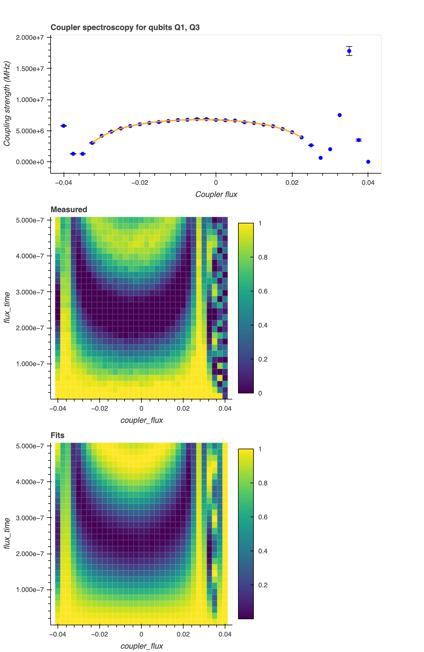
Fitting Rabi Oscillations to the experimental trace (
populationversusflux_timefor eachcoupler_fluxes). The function is \(f(x) = 1 - (g/\Omega)^{2} \sin^2(\Omega x)\). Here, \(\Omega = \sqrt{g^2 + \delta^2}\) corresponds to the Rabi frequency, i.e., the frequency at which the probability amplitudes of two energy levels fluctuate in an oscillating electromagnetic field. \(\delta\) is the detuning frequency (delta), and \(g\) is the qubit-qubit coupling strength (g12). -
Determining the bare qubit-qubit coupling (now referred to as
g12) by fitting a quadratic line shape to the spectroscopy trace (deltaversuscoupler_fluxes). The fitting function, denoted as \(f(x)\), exhibits a quadratic dependence on the flux, i.e., \(f(x) = 1 / (cx^2 + bx + a + g)\), where \(x\) represents thecoupler_fluxes, and \(g\) representsg12.
-
Fei Yan, Philip Krantz, Youngkyu Sung, Morten Kjaergaard, Daniel L. Campbell, Terry P. Orlando, Simon Gustavsson, and William D. Oliver. Tunable coupling scheme for implementing high-fidelity two-qubit gates. Phys. Rev. Appl., 10:054062, Nov 2018. doi:10.1103/PhysRevApplied.10.054062. ↩