Calibrate $\frac{\pi}{2}$ amplitude with ping-pong

This experiment uses ping-pong to calibrate the amplitude of an $R_{x}(\frac{\pi}{2})$ gate.

Description

Precisely estimating a very small error on a control parameter requires a technique that can selectively amplify the error of interest. To do this, we use the ping-pong technique, which uses error amplification to correct over- or under-rotations in single-qubit gates¹.

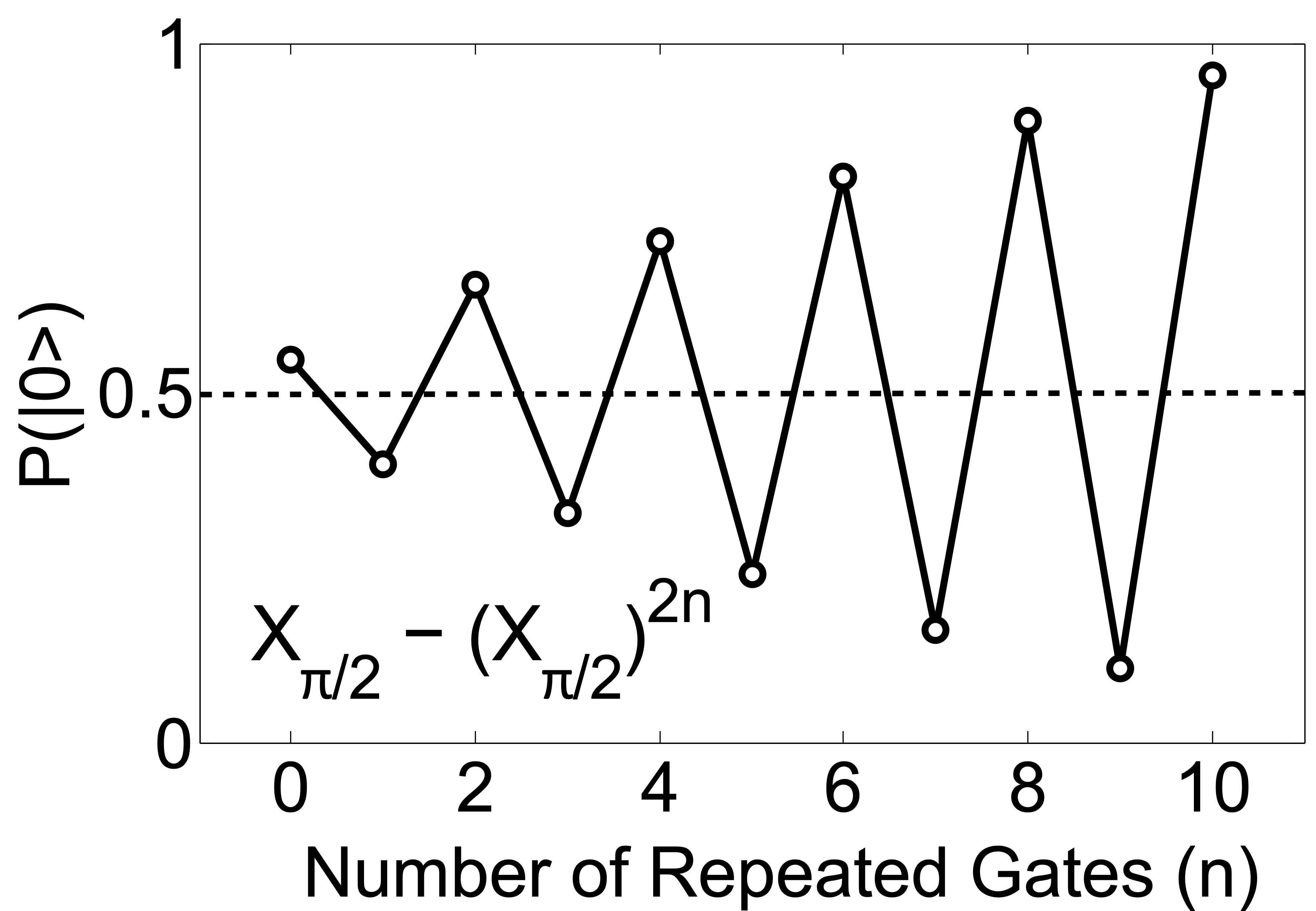
In this experiment, the $\frac{\pi}{2}$ pulse ($R_{x}(\frac{\pi}{2})$ gate) is tuned by repeating the pulse in the sequence [$R_{x}(\frac{\pi}{2})$ - $(R_{x}(\frac{\pi}{2}))^{2n}$]. The first $\frac{\pi}{2}$-pulse prepares the qubit in the superposition state $\frac{1}{\sqrt{2}}(|0\rangle +|1\rangle)$. This is important since error amplification experiments are most sensitive to angle errors when we measure points along the equator of the Bloch sphere.

If the $\frac{\pi}{2}$ pulse is perfectly calibrated, the qubit will return to a superposition state (equator of the Bloch sphere) at the end of the sequence. If there are slight miscalibrations, the qubit state will be either above or below the equator and this error will be amplified with increasing values of $n$, as can be seen in the figure below.

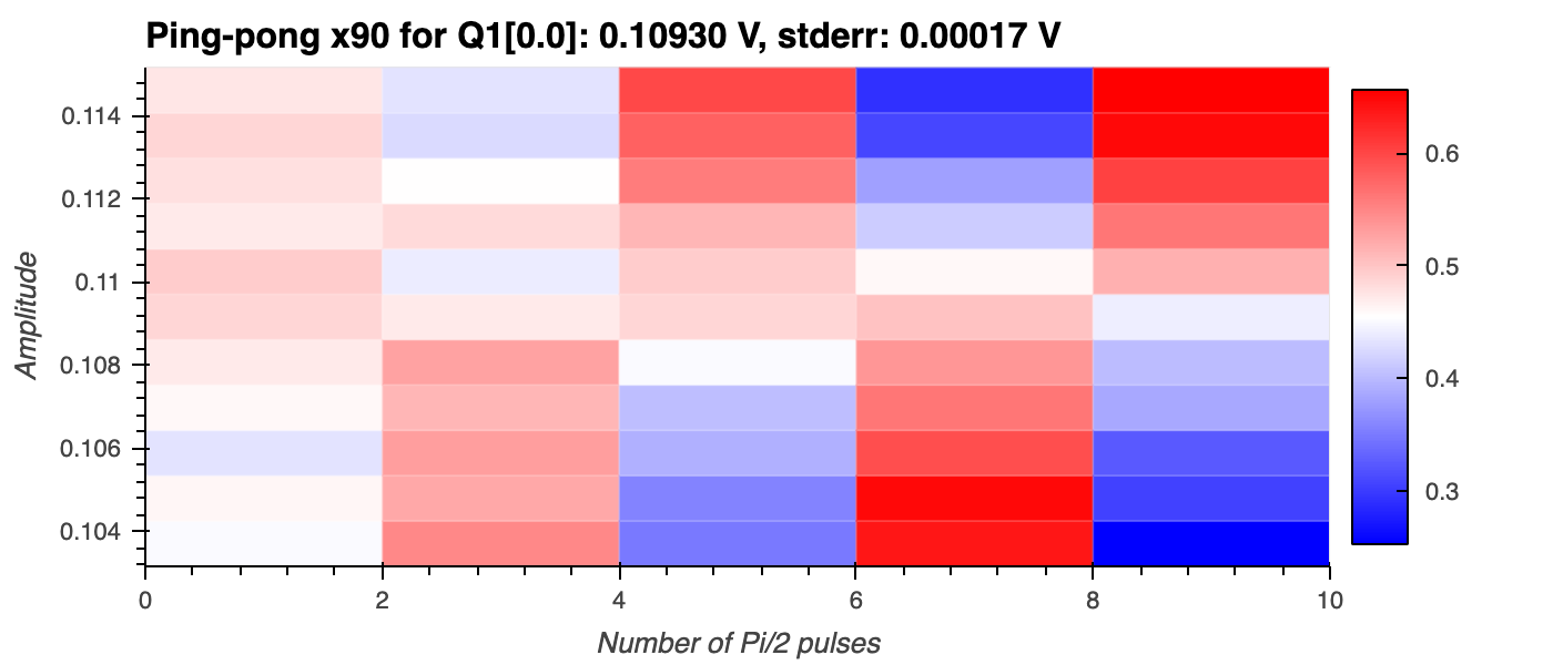
Over- and under-rotations are estimated by fitting the measured population of the qubit ground state, $P(|0\rangle)$, which varies as a function of $n$ and the relative pulse amplitude, $x$. The fit roughly follows the general relation:

$$f(x, n) = -a \cos(x(d\theta + \varphi_{\text{gate}}) n + \varphi_{0}) + b .$$

Here, $d\theta$, $a$, and $b$ are fit parameters, where $d\theta$ represents the angle of over- or under-rotation, and $a$ and $b$ denote the amplitude and $y$-offset of the cosine fit function, respectively.

The parameters $\varphi_{\text{gate}}$ and $\varphi_{0}$ are fixed, with $\varphi_{\text{gate}}$ being the gate angle (in this case, $\frac{\pi}{2}$) and $\varphi_{0}$ being the initial phase offset (which is $\frac{\pi}{2}$ due to the initial $R_{x}(\frac{\pi}{2})$ gate).

Experiment steps

1. The sequence [$\frac{\pi}{2}$-pulse − [$\frac{\pi}{2}$-pulse]$^{2n}$] is applied to the qubit while sweeping the $\frac{\pi}{2}$-amplitude, $x$, over a range of values defined around the expected amplitude.

2. The resonator transmission is measured for each value of the $\frac{\pi}{2}$-amplitude.

3. Steps 1 and 2 are repeated, increasing the number of repetitions $n$.

Analysis steps

1. The qubit state is predicted from the $I$-$Q$ data by applying the discriminator trained in the Readout Discriminator Training experiment.

2. The over- or under- rotation, $d\theta$, is determined by fitting a cosine function to the qubit ground state populations.

3. The optimal $\frac{\pi}{2}$-pulse amplitude is then obtained by scaling the uncalibrated pulse using the factor $\frac{\varphi_{\text{gate}}}{\varphi_{\text{gate}} + d\theta}$.

---

1. Sarah Sheldon, Lev S. Bishop, Easwar Magesan, Stefan Filipp, Jerry M. Chow, and Jay M. Gambetta. Characterizing errors on qubit operations via iterative randomized benchmarking. Phys. Rev. A, 93:012301, Jan 2016. doi:10.1103/PhysRevA.93.012301. ↩